15 Ways to Create a Document-Term Matrix in R
Original post on December 2020. Updated on August 2021.
The Document-Term Matrix (DTM) is the foundation of computational text analysis, and as a result there are several R packages that provide a means to build one. What is a DTM? It is a matrix with rows and columns, where each document in some sample of texts (called a corpus) are the rows and the columns are all the unique words (often called types or vocabulary) in the corpus. The cells of the matrix are typically a count of how many times each unique word occurs in a given document (often called tokens).
Below, I attempt a comprehensive overview and comparison of 15 different methods for creating a DTM. Two are custom functions written in base R. The rest are from eleven text analysis packages. One of these is an R package, text2map, that I developed with Marshall Taylor (Stoltz and Taylor 2022). (The dtm_builder() function was developed in tandem with writing the original comparison back in December 2020).
Below are the non-text analysis packages we’ll be using.
library(tidyverse)
library(ggpubr)
library(Matrix)
library(slam)
library(bench)
And, here are the text analysis R packages we’ll be using. These include every single package that includes functions to create DTM that I could find (the koRpus package does provide a document-term matrix method, but I could not get it to work). Feel free to let me know if I’ve missed a package that creates a DTM.
packages <- c("tidytext",
              "tm",
              "quanteda",
              "text2map",
              "text2vec",
              "textTinyR",
              "corpustools",
              "textmineR",
              "wactor",
              "gofastr",
              "udpipe")
#install.packages(packages)
invisible(lapply(packages, library, character.only = TRUE))
Getting Started #
We need some text data! Let’s get scripts from Star Trek from the rtrek package, because, why not? Let’s create a corpus for all series, and then a corpus of just Star Trek: The Next Generation. We will filter the scripts by series, and then collapse each line so it is one script per episode.
df.trek <- rtrek::st_transcripts() |>
    unnest(cols = c(text) ) |>
    filter(!is.na(line)) |>
    group_by(series, number) |>
    summarize(text = paste0(line, collapse = " "),
              doc_id = first(title),
              season = first(season),
              airdate = first(airdate)) |> ungroup()

df.tng <- rtrek::st_transcripts() |>
    unnest(cols = c(text) ) |>
    filter(series == "TNG") |> # limit to TNG
    filter(!is.na(line)) |>
    group_by(number) |>
    summarize(text = paste0(line, collapse = " "),
              doc_id = first(title),
              season = first(season),
              airdate = first(airdate)) |> ungroup()
Let’s do a tiny bit of preprocessing (lowercasing, smooshing contractions, removing punctuation, numbers, and getting rid of extra spaces).
df.trek <- df.trek |>
  dplyr::mutate(
      clean_text = tolower(text),
      clean_text = gsub("[']", "", clean_text),
      clean_text = gsub("[[:punct:]]", " ", clean_text),
      clean_text = gsub('[[:digit:]]+', " ", clean_text),
      clean_text = gsub("[[:space:]]+", " ", clean_text),
      clean_text = trimws(clean_text))
df.tng <- df.tng |>
  dplyr::mutate(
      clean_text = tolower(text),
      clean_text = gsub("[']", "", clean_text),
      clean_text = gsub("[[:punct:]]", " ", clean_text),
      clean_text = gsub('[[:digit:]]+', " ", clean_text),
      clean_text = gsub("[[:space:]]+", " ", clean_text),
      clean_text = trimws(clean_text))
Base R, Dense DTMs #
To get started, let’s create two base R methods for creating dense DTMs. There are three necessary steps: (1) tokenize, (2) create vocabulary, and (3) match and count.
First, each document is split into list of individual tokens. Second, from these lists of tokens, we need to extract only the unique tokens to create a vocabulary. Finally, we will count each time we find a match between a token in a document with a token in the vocabulary.
While the above are essential, there are a few optional steps which functions may or may not take by default. First, the most basic DTM uses the raw counts of each word in a document. Some functions may include the option to weight the matrix. The most common is to normalize by the row count to get relative frequencies. Since all weightings require raw counts anyway, we will just stop at a count DTM (not to mention relative frequencies will turn an integer matrix into a real number matrix, which will result in a larger object in terms of memory).
Second, the columns of our DTM may be sorted by (1) the order they appear in the corpus, (2) alphabetic order, or (3) by their frequency in the corpus. The first option will be the fastest and the third option being the slowest. The function may also incorporate the removal or “stopping” of certain tokens. It is more efficient to build the DTM first, and then simply remove the columns that match a given stoplist.
Finally, we can tokenize using a variety of rules. Both methods below will use strsplit() with a literal, single space (fixed = TRUE significantly speeds up this process). This is a very simple tokenizing rule. This also means it is very fast in comparison to more complex rules. For example, we could tokenize by every two word bi-gram or instead of a literal single space, we could use other kinds of whitespace (tabs, carriage returns, newlines, etc…). Both methods below will also use unique() for getting the unique tokens (i.e. vocabulary) of the corpus.
base_loop <- function(text, doc_id){
    tokns <- strsplit(text, " ", fixed=TRUE)
    vocab <- sort(unique(unlist(tokns)))
    dtm <- matrix(data = 0L,
                  ncol = length(vocab), nrow = length(tokns),
                  dimnames = list(doc_id, vocab) )
    freqs <- lapply(tokns, table)
    for (i in 1:length(freqs) ){
                doc <- freqs[[i]]
                dtm[i, names(doc)] <- as.integer(doc)
    }
    return(dtm)
}
base_lapply <- function(text, doc_id){
    tokns <- strsplit(text, " ")
    vocab <- sort(unique(unlist(tokns)))
    FUN <- function(x, lev){tabulate(factor(x, levels = lev,
                                            ordered = TRUE),
                                            nbins = length(lev))}
    out <- lapply(tokns, FUN, lev = vocab)
    dtm <- as.matrix(t(do.call(cbind, out) ) )
    dimnames(dtm) <- list(doc_id, vocab)
    return(dtm)
}
The first function uses a for loop with the table function to count the number of instances of a given token and the second uses only lapply with the tabulate function to count tokens. In base R, matrices are represented in a “dense” format, which is given the class matrix – this will make more sense when we discuss sparsity below. Generally, lapply is more efficient, however, because we initialize an empty matrix (and thus preallocate memory) and then fill it up with the first function, our for loop approach may perform better.
dtm1 <- dtm_base_loop(df.trek$clean_text, df.trek$doc_id)
dtm2 <- dtm_base_lapply(df.trek$clean_text, df.trek$doc_id)
Let’s double check that these two methods produced identical results. We’ll (1) check that they’re the same dimensions, (2) check they sum to the same number of total tokens in the corpus, (3) and check that the words and document IDs (episode titles) are the same.
dim(dtm1) == dim(dtm2)
sum(dtm2) == sum(dtm1)
dimnames(dtm1) %in% dimnames(dtm2)
Which method is more efficient? To compare methods, I will use the mark() function from the bench package.
df.mark <- bench::mark(
    dtm_bloop <- base_loop(df.trek$clean_text, df.trek$doc_id),
    dtm_blapply <- base_lapply(df.trek$clean_text, df.trek$doc_id),
    check = FALSE,
    iterations = 10,
    memory = TRUE
    )
df.mark |>
    mutate(expression = c("loop", "lapply")) |>
    select(expression, mem_alloc, median)
#
| expression   | mem_alloc   | median   |
|:------------:|:-----------:|:--------:|
|loop          |       1.06GB|     3.58s|
|lapply        |       2.36GB|     6.37s|
Similar, but our for loop function beat the lapply. It’s possible that with a larger corpus lapply will show more substantial gains over the for loop method.
Sparse DTMs #
As a result of the nature of language, DTMs tend to be very “sparse” —meaning, they have lots and lots of zeros. For example, let’s see how many cells are zeros in one of the dense DTMs we just created based on Star Trek: TNG scripts.
total.cells <- ncol(dtm1) * nrow(dtm1)
zero.cells  <- sum(dtm1==0)
zero.cells/total.cells
## [1] 0.9440146
That is a lot of zero cells! The two functions above produced a basic “dense” matrix, which can quickly take up a lot of memory. There are several strategies for dealing with the memory issues of very large matrices in R, but, for the most part you will need enough RAM on your machine to hold the entirety of the matrix in memory at once. The most straightforward way to deal with memory limitations is to simply represent a matrix as a slightly different kind of data object called a “sparse” matrix. Simply put, when a matrix has a lot of zeros, the sparse format will produce a smaller object. Many of the dedicated DTM functions use this format, so let’s dive a little deeper into them.
There are two popular R packages that offer sparse matrix formats, Matrix and slam. The latter package offers one main kind of sparse matrix called a simple_triplet_matrix. The former package has several more. We will use the dgCMatrix class to represent integer and real number DTMs and lgCMatrix for the binary DTM (the Matrix package also has a triplet format: dgTMatrix).
We built text2map’s dtm_builder() first for speed, and second for memory efficiency. We were able to speed up the vocabulary creation step and the matching and counting step. And, just like the previous functions, we also limit tokenizing to the fixed, literal space.
Comparing DTM Functions #
Now that we have a better understanding of what is happening “under the hood” when creating a DTM in R, we can turn to comparing how well dedicated text analysis packages produce DTMs. We will measure the time and memory used to turn our lightly pre-processed Star Trek scripts into a DTM.
The dedicated functions all use either dgCMatrix or simple_triplet_matrix formats to represent the final outputs, but several intermediary steps are taken prior. This often involves converting the texts into different kinds of data structures. For example, in both our base R functions, we turn each individual episode into a list of each individual token, then we turn that into a list of token counts. A popular package, tidytext, uses the tokenizers package and then outputs a three-column token-count data frame, where each row is a document, term, and value – also called a tripletlist. Next, we can use cast_dtm() to get the equivalent to the tm package’s dtm or cast_dfm() to produce the equivalent to the quanteda package’s dfm. The udpipe package also creates a tripletlist before creating a DTM.
Next, we’ll create a unique function for each of the different packages that will go directly from lightly cleaned text to a DTM. Because a lot of these packages use the same or similar nomenclature, we will use the explicit package declaration for each function (::).
tm_dtm <- function(text){
        dtm  <- tm::DocumentTermMatrix(tm::VCorpus(
                    tm::VectorSource(text)),
                    control = list(wordLengths = c(1, Inf)))
}
quanteda_dfm <- function(text){
        dfm <- quanteda::dfm(quanteda::tokens(text, what = "fastestword"))
}
tidytext_dtm <- function(df.text) {
        dtm <- df.text |>
            tidytext::unnest_tokens(word, clean_text) |>
            dplyr::count(doc_id, word, sort = TRUE) |>
            tidytext::cast_dtm(doc_id, word, n)
}
tidytext_dfm <- function(df.text) {
        dfm <- df.text |>
            tidytext::unnest_tokens(word, clean_text) |>
            dplyr::count(doc_id, word, sort = TRUE) |>
            tidytext::cast_dfm(doc_id, word, n)
}
corpustools_dtm <- function(df.text){
        tc <- corpustools::create_tcorpus(df.text,
        doc_col='doc_id', ext_columns = 'clean_text')
        dtm <- corpustools::get_dtm(tc, 'token')
}
corpustools_dfm <- function(df.text){
        tc <- corpustools::create_tcorpus(df.text,
        doc_col='doc_id', text_columns = 'clean_text')
        dfm <- corpustools::get_dfm(tc, 'token')
}
text2vec_dtm <- function(text){
        tokens <- text2vec::itoken(text, sep = " ", xptr = FALSE)
        vocab  <- text2vec::create_vocabulary(tokens)
        dtm <- text2vec::create_dtm(tokens, text2vec::vocab_vectorizer(vocab))
}
textminer_dtm <- function(text, doc_id){
        dtm <- textmineR::CreateDtm(doc_vec = text,
                                    doc_names = doc_id, stopword_vec = NULL,
                                    remove_punctuation = FALSE,
                                    remove_numbers = FALSE,
                                    verbose = FALSE, cpus = 1)
}
texttinyr_dtm <- function(text){
        init <- textTinyR::sparse_term_matrix$new(
                                  vector_data = text,
                                  document_term_matrix = TRUE)
        dtm <- init$Term_Matrix(sort_terms = TRUE,
                                  split_string = TRUE,
                                  tf_idf = FALSE, verbose = FALSE)
}
wactor_dtm <- function(text){
        dtm <- wactor::dtm( wactor::wactor(text, max_words = Inf))
}
gofastr_dtm <- function(text){
        dtm <- gofastr::q_dtm(text, keep.hyphen = FALSE, to = "tm")
}
udpipe_dtm <- function(text, doc_id){
        dtm <- udpipe::document_term_matrix(
               udpipe::document_term_frequencies(text, document = doc_id) )
}
We use our two base R functions as baselines, along with the dtm_builder() function from our text2map package. Then we use the two most commonly used packages, tm and quanteda. By default these two output a simple_triplet_matrix and a dgCMatrix matrix, respectively. Next, we will use tidytext and corpustools which both provide methods of producing matrices compatible with the tm and quanteda packages. The next group of five packages are explicitly oriented toward optimization (note: as of writing, gofastr and wactor have not been updated in a while). Finally, there is udpipe, which is particularly well known for providing parsers for numerous non-English languages. Together, we will compare 15 different methods.
df.mark.tng <- bench::mark(
    dtm_01 <- base_loop(df.tng$clean_text, df.tng$doc_id),
    dtm_02 <- base_lapply(df.tng$clean_text, df.tng$doc_id),
    dtm_03 <- text2map::dtm_builder(df.tng, clean_text, doc_id),
    dtm_04 <- tm_dtm(df.tng$clean_text),
    dtm_05 <- quanteda_dfm(df.tng$clean_text),
    dtm_06 <- tidytext_dtm(df.tng),
    dtm_07 <- tidytext_dfm(df.tng),
    dtm_08 <- corpustools_dtm(df.tng),
    dtm_09 <- corpustools_dfm(df.tng),
    dtm_10 <- text2vec_dtm(df.tng$clean_text),
    dtm_11 <- textminer_dtm(df.tng$clean_text, df.tng$doc_id),
    dtm_12 <- texttinyr_dtm(df.tng$clean_text),
    dtm_13 <- wactor_dtm(df.tng$clean_text),
    dtm_14 <- gofastr_dtm(df.tng$clean_text),
    dtm_15 <- udpipe_dtm(df.tng$clean_text,df.tng$doc_id),
    check = FALSE,
    iterations = 100,
    memory = TRUE
)
Now, we ran 100 iterations using the bench package. We can turn the output into violin plots to show the overall range in terms of time, and we can plot a bar chart to show the overall memory allocated during each iteration.
df.plot <- df.mark.tng |>
    mutate(expression = c("base (loop)", "base (lapply)", "text2map",
                          "tm", "quanteda",
                          "tidytext (tm)", "tidytext (qu)",
                          "corpustools (tm)", "corpustools (qu)",
                          "text2vec", "textminer", "texttinyr",
                          "wactor", "gofastr", "udpipe") )p.time <- df.plot |>
    tidyr::unnest(c(time, gc) ) |>
    mutate(Function = fct_reorder(expression, median)) |>
    ggplot(aes(Function, time, fill = Function)) +
    geom_violin() +
    guides(fill = "none") +
    coord_flip() +
    labs(title = "Converting Star Trek Episodes to DTM, The Next Generation",
         caption = "")
p.memo <- df.plot |>
    mutate(Kbs = as.numeric(mem_alloc)/1024,
           Mbs = as.numeric(Kbs)/1024,
           Function = fct_reorder(expression, Mbs)) |>
    ggplot(aes(Function, Mbs, fill = Function)) +
    geom_bar(stat="identity", position = position_dodge(width = 0.8) ) +
    guides(fill = "none") +
    coord_flip() +
    labs(title = "",
         caption = "Source: Dustin Stoltz (2021) | www.dustinstoltz.com")

The text2map function dtm_builder() is the fastest – which was to be expected since we built it specifically for this purpose. As far as the other text analysis packages go, the winner, in terms of being fast and memory efficient is text2vec. textTinyR is written almost entirely in Rcpp, meaning that it is very memory efficient, but seems to lose some time interfacing between R and C++. tidytext loses a lot of time because it first creates a tripletlist tibble, then creates a DTM (our base R loop function beats it in terms of speed and almost ties it in terms of memory despite operating on a base R dense matrix). In terms of the two most popular packages, quanteda edges out the tm package.
It’s important to note that these packages may use different tokenizing rules or remove some kinds of words by default. I attempted to standardize this across each function as best I could, but two functions produce a DTM of a different size from the rest. The tm option in corpustools produced a DTM with 25,583 words, while the gofastr package produced a DTM with only 13,096 words. I was unable to figure out what was up with these two packages.
Furthermore, these tests are all creating a DTM with 176 episodes and a vocabulary of 20,858 words. Perhaps varying these parameters would change the rankings. So, let’s look at every Star Trek episode across all series, totalling 716 episodes and 39,324 unique words (er, 50,805 for corpustools’ tm option and 24,994 words for gofastr). Note: this may take a while for most personal computers.
df.mark.all <- bench::mark(
    dtm_01 <- base_loop(df.trek$clean_text, df.trek$doc_id),
    dtm_02 <- base_lapply(df.trek$clean_text, df.trek$doc_id),
    dtm_03 <- text2map::dtm_builder(df.trek, clean_text, doc_id),
    dtm_04 <- tm_dtm(df.trek$clean_text),
    dtm_05 <- quanteda_dfm(df.trek$clean_text),
    dtm_06 <- tidytext_dtm(df.trek),
    dtm_07 <- tidytext_dfm(df.trek),
    dtm_08 <- corpustools_dtm(df.trek),
    dtm_09 <- corpustools_dfm(df.trek),
    dtm_10 <- text2vec_dtm(df.trek$clean_text),
    dtm_11 <- textminer_dtm(df.trek$clean_text, df.trek$doc_id),
    dtm_12 <- texttinyr_dtm(df.trek$clean_text),
    dtm_13 <- wactor_dtm(df.trek$clean_text),
    dtm_14 <- gofastr_dtm(df.trek$clean_text),
    dtm_15 <- udpipe_dtm(df.trek$clean_text, df.trek$doc_id),
    check = FALSE,
    iterations = 100,
    memory = TRUE
)
df.plot <- df.mark.all |>
    mutate(expression = c("base (loop)", "base (lapply)", "text2map",
                          "tm", "quanteda",
                          "tidytext (tm)", "tidytext (qu)",
                          "corpustools (tm)", "corpustools (qu)",
                          "text2vec", "textminer", "texttinyr",
                          "wactor",  "gofastr", "udpipe") )
p.time <- df.plot |>
    tidyr::unnest(c(time, gc) ) |>
    mutate(Function = fct_reorder(expression, median)) |>
    ggplot(aes(Function, time, fill = Function)) +
    geom_violin() +
    guides(fill = "none") +
    coord_flip() +
    labs(title = "Converting Star Trek Episodes to DTM, All Series",
         caption = "")
p.memo <- df.plot |>
    mutate(Kbs = as.numeric(mem_alloc)/1024,
           Mbs = as.numeric(Kbs)/1024,
           Function = fct_reorder(expression, Mbs)) |>
    ggplot(aes(Function, Mbs, fill = Function)) +
    geom_bar(stat="identity", position = position_dodge(width = 0.8) ) +
    guides(fill = "none") +
    coord_flip() +
    labs(title = "",
         caption = "Source: Dustin Stoltz (2021) | www.dustinstoltz.com")
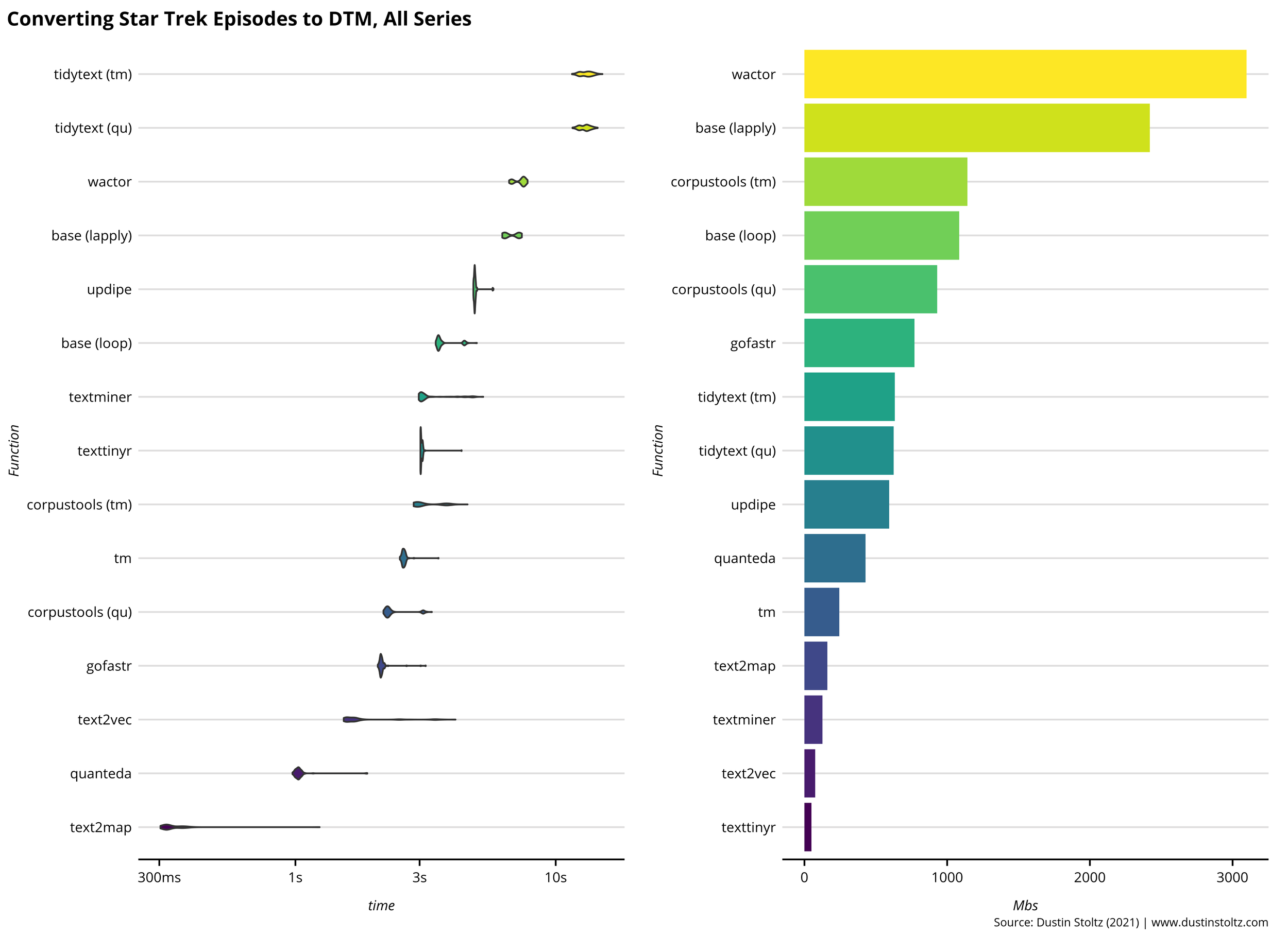
With a much larger corpus, the ranks stay remarkably similar. Our text2map function is hovering at the fastest end with around 300 milliseconds to create this DTM, followed by quanteda and text2vec. textTinyR still has that time overhead, but beats every other function in overall memory allocated. tidytext continues to offer by far the slowest DTM creation, and middle of the pack in terms of memory.
References #
Stoltz, Dustin S., and Marshall A. Taylor. (2022). “text2map: R tools for text matrices.” Journal of Open Source Software 7(72), 3741
Notes #
For the plot aesthetics, I used the following:
devtools::install_gitlab("culturalcartography/ggastrum")
ggastrum::set_theme()